目录

• 前言
• 总体设计
• • 系统整体结构图
  • 系统流程图
• 运行环境
• • 1. 硬件环境
  • 2. Python 环境
• 模块实现
• • 1. 数据预处理
  • 2. 数据加载
  • 3. 模型构建
  • 4. 模型训练及保存
  • 5. 模型加载与调用
• 系统测试
• • 1. 模型准确率
  • 2. 分类别准确率
• 工程源代码下载
• 其它资料下载

前言

本项目基于Faster R-CNN模型，通过RPN网络（Region Proposal Network）获取图片中的候选区域，并利用RestNet50模型提取特征，旨在实现对生活垃圾的智能分拣。

在该项目中，我们使用Faster R-CNN模型，它是一种经典的目标检测算法，能够同时进行物体检测和区域提议。通过RPN网络，我们能够在输入图片中快速识别出潜在的候选区域，这些区域可能包含生活垃圾物品。

接下来，我们使用RestNet50模型进行特征提取。RestNet50是一种深度卷积神经网络，具有较强的特征提取能力。我们将候选区域输入RestNet50模型，提取出高维特征表示，以捕捉垃圾物品的关键信息。

通过将候选区域和其对应的特征输入到后续的分类器中，我们可以对生活垃圾进行智能分拣。分类器可以根据特征表示判断每个候选区域属于哪一类垃圾，例如可回收物、厨余垃圾、有害垃圾等，实现智能化的垃圾分类过程。

本项目的目标是利用Faster R-CNN模型和RestNet50模型的结合，通过智能化的图片分析和特征提取，实现对生活垃圾的智慧分拣。这项技术有助于提高垃圾处理的效率和准确性，为环境保护和资源回收做出贡献。

总体设计

本部分包括系统整体结构图和系统流程图。

系统整体结构图

系统整体结构如图所示。

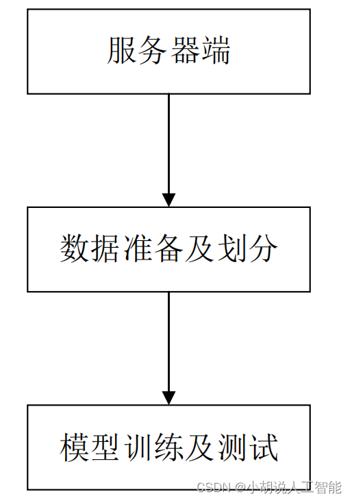
系统流程图

系统流程如图所示。

运行环境

本部分包括硬件环境和 Python 环境。

1. 硬件环境

FasterRCNN 对计算要求较高，有一部分是 Restnet50 的卷积层。必须使用较大内存的GPU 才可以完成训练。在本项目中，用华为云提供的模型训练服务（GPU tesla P100)实现，链接:https://www.hwtelcloud.com/products/mts。

2. Python 环境

使用软件的主要版本如下：

模块实现

本项目包括 5 个模块：数据预处理、数据加载、模型构建、模型保存及训练、模型加载及调用，下面分别给出各模块的功能介绍及相关代码。

1. 数据预处理

数据下载地址： https://pan.baidu.com/s/1ZAbzYMLv0fcLFJsu64u0iw，提取码：yba3

数据信息被存储在 json 文件中，使用 python 和 jupyter notebook 对 json 文件进行解析，并进行数据探索。经过分析，获取的垃圾数据集中单类垃圾共有 80000 张训练集图片，204种分类。且每种分类的垃圾图片数量基本相同，约为 300 张左右。由于时间短，仅使用了10种类别的单类图片用于训练和验证，这 10 种类别分别是瓜子壳、核桃、花生壳、面包、饼干、菌菇类、菜叶、菜根、甘蔗皮、中药材、枣核。其中训练集有 3000 张，测试集有843张，如图所示。

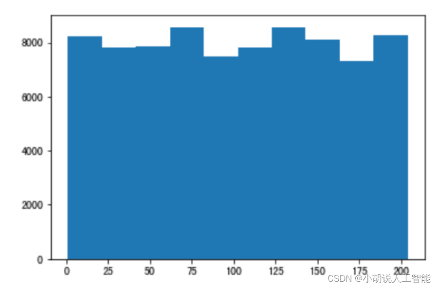
由于 FasterRCNN 使用 anchor 机制，即锚框。需要获取样本尺寸信息作为先验信息，设计锚框。因此，使用 matplotlib 绘制出关于样本尺寸的散点图和直方图。如图1～图 3 所示。

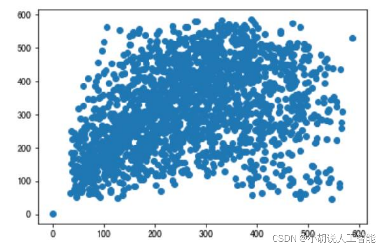
锚框机制，需要预先提供九个不同尺寸的锚框，应尽量贴合目标的尺寸。使用 K-means算法进行聚类，获得合适的锚框，如下图所示。

#使用KMeans确定anchor的长宽
from sklearn.cluster import KMeans
from sklearn.externals import joblib
data=np.hstack((np.array(widths).reshape((-1,1)),np.array(heights).reshape((-1,1))))
clf = KMeans(n_clusters=9)
s = clf.fit(data)
centers=clf.cluster_centers_
plt.scatter(widths,heights,alpha=0.2)
plt.scatter([i[0] for i in centers ],[i[1] for i in centers ],c='r')

结合Kmeans结果，并进行手动调整，可以设计锚框尺寸。

#锚框尺寸self.anchor_box_scales = [150, 300, 435]#锚框比例self.anchor_box_ratios = [[1, 1], [1, 0.91], [1, 1.25]]

2. 数据加载

本项目使用 biendata(https://biendata.com/)的一个比赛，2020 海华 AI 挑战赛垃圾分类。这个比赛，与华为模型训练服务合作，可以直接在华为模型训练平台上下载、读取训练比赛数据。

使用 github 上提供基于 Keras 的 FasterRCNN 模型。该模型需要将图片信息以 VOC2012数据集的格式进行存储，将图片信息转为该格式，代码写在 garbage_dataset.py 中。

  def w_voc(self):#将目标的信息写入voc格式数据集中data_path = 'VOC2012'print("将目标的信息写入voc格式数据集中")#annot_path是存放目标信息xml文件的文件夹annot_path = os.path.join(data_path, 'Annotations_single')#imgs_path是存放图片的文件夹位置#imgs_path = os.path.join(data_path, 'JPEGImages')#imgset_path是存放图片名的文件夹imgsets_path_trainval = os.path.join(data_path, 'ImageSets', 'single', 'trainval.txt')annot_indexs=0#用来标记新图片的起始目标信息位置if os.listdir(annot_path) != None:os.system('rm -f '+annot_path+'/*')with open(self.json_dir,'r',encoding='utf-8') as fp:self.json_dict = json.load(fp)with open(imgsets_path_trainval,'w') as fp:#将图片名存入imgsets中for img in self.json_dict['images']:fp.write(img['file_name'].split('/')[1]+'\n')for img in self.json_dict['images']:annots=[]file_name=img['file_name'].split('/')[1]xml_name=file_name.split('.')[0]+'.xml'for annot in self.json_dict['annotations'][annot_indexs:]:
#获取每张图片下的目标信息if str(annot['image_id'])==file_name.split('.')[0]:annots.append(annot)annot_indexs+=1#更新目标信息索引else:break#将图片信息与目标信息写入xml文件中,并存入annotations文件夹

在 FasterRCNN 中对 VOC 格式数据读取代码存在 keras_frcnn/pascal_voc_parser.py。再通 过 keras_frcnn/data_augment.py 读 取 每 一 张 图 片 信 息 和 相 应 目 标 信 息 ，keras_frcnn/data_generators.py 作为发生器。

3. 模型构建

数据加载进模型之后，需要定义模型结构，并优化损失函数。

1）定义模型结构

从keras_frcnn/resnet.py 调用相关的模型层。

from keras_frcnn import resnet as nn
#定义基本网络（此处为Resnet，可以是VGG，Inception等）
shared_layers = nn.nn_base(img_input, trainable=True)
#定义RPN，建立在基础层上
num_anchors=len(cfg.anchor_box_scales)* len(cfg.anchor_box_ratios)
rpn = nn.rpn(shared_layers, num_anchors)
classifier = nn.classifier(shared_layers, roi_input, cfg.num_rois, 	nb_classes=len(classes_count), trainable=True)
model_rpn = Model(img_input, rpn[:2])
model_classifier = Model([img_input, roi_input], classifier)
#这是一个同时包含RPN和分类器的模型，用于加载/保存模型的权重
model_all = Model([img_input, roi_input], rpn[:2] + classifier)

2. 损失函数及模型优化

#优化器
optimizer = Adam(lr=1e-5)
optimizer_classifier = Adam(lr=1e-5)
model_rpn.compile(optimizer=optimizer,
loss=[losses_fn.rpn_loss_cls(num_anchors), 			losses_fn.rpn_loss_regr(num_anchors)])
model_classifier.compile(optimizer=optimizer_classifier,
loss=[losses_fn.class_loss_cls, 			losses_fn.class_loss_regr(len(classes_count)-1)],                           
metrics={'dense_class_{}'.format(len(classes_count)):'accuracy'})
model_all.compile(optimizer='sgd', loss='mae')

4. 模型训练及保存

本部分包括模型训练和模型保存。

1）模型训练

#相关参数
epoch_length = 1000
num_epochs = int(cfg.num_epochs)
iter_num = 0
#调用模型进行训练X, Y, img_data = next(data_gen_train)loss_rpn = model_rpn.train_on_batch(X, Y)             P_rpn = model_rpn.predict_on_batch(X)

2）模型保存

model_all.save_weights(cfg.model_path)
mox.file.copy(cfg.model_path, 	os.path.join(Context.get_model_path(), 'model_frcnn.vgg.hdf5'))

5. 模型加载与调用

Keras 需要先将网络定义好，才能加载模型。相关代码在 test_frcnn_kitti.py 中

1）模型加载

#定义RPN，建立在基础层上		num_anchors=len(cfg.anchor_box_scales)*len(cfg.anchor_box_ratios)
rpn_layers = nn.rpn(shared_layers, num_anchors)
classifier=nn.classifier(feature_map_input,roi_input, cfg.num_rois, 	nb_classes=len(class_mapping),trainable=True)
model_rpn = Model(img_input, rpn_layers)
model_classifier_only=Model([feature_map_input,roi_input],classifier)
model_classifier= Model([feature_map_input, roi_input], classifier)
print('Loading weights from {}'.format(cfg.model_path))
model_rpn.load_weights(cfg.model_path, by_name=True)
model_classifier.load_weights(cfg.model_path, by_name=True)
model_rpn.compile(optimizer='sgd', loss='mse')
model_classifier.compile(optimizer='sgd', loss='mse')

2）模型测试

def predict_single_image(img_path, model_rpn, model_classifier_only, cfg, class_mapping):#将空间金字塔池应用于建议的区域boxes = dict()for jk in range(result.shape[0] // cfg.num_rois + 1):rois = np.expand_dims(result[cfg.num_rois * jk:cfg.num_rois * (jk + 1), :], axis=0)if rois.shape[1] == 0:breakif jk == result.shape[0] // cfg.num_rois:curr_shape = rois.shapetarget_shape = (curr_shape[0], cfg.num_rois, curr_shape[2])rois_padded = np.zeros(target_shape).astype(rois.dtype)rois_padded[:, :curr_shape[1], :] = roisrois_padded[0, curr_shape[1]:, :] = rois[0, 0, :]rois = rois_padded[p_cls, p_regr] = model_classifier_only.predict([F, rois])for ii in range(p_cls.shape[1]):if np.max(p_cls[0, ii, :]) < bbox_threshold or np.argmax(p_cls[0, ii, :]) == (p_cls.shape[2] - 1):continuecls_num = np.argmax(p_cls[0, ii, :])if cls_num not in boxes.keys():boxes[cls_num] = [](x, y, w, h) = rois[0, ii, :]try:(tx, ty, tw, th) = p_regr[0, ii, 4 * cls_num:4 * (cls_num + 1)]tx /= cfg.classifier_regr_std[0]ty /= cfg.classifier_regr_std[1]tw /= cfg.classifier_regr_std[2]th /= cfg.classifier_regr_std[3]x, y, w, h = roi_helpers.apply_regr(x, y, w, h, tx, ty, tw, th)

系统测试

本部分包括模型准确率和分类别准确率。

1. 模型准确率

通过华为模型训练平台对模型进行测试，并写入result.txt文件中存储，相关代码如下：

true_count=0#使用测试集进行准确度的测试,并存入文件中
with open('./val_single.txt','r') as f:
val_data=f.readlines()
img_count=len(val_data)for index,val in enumerate(val_data):if index%50 ==0:K.clear_session()test_cls=predict(val.split()[0])if int(test_cls)==int(val.split()[1]):true_count+=1with open('/cache/result.txt','a') as f: 
f.write("%s %s %s\n"%(val.split()[0],val.split()[1],test_cls))    accuray=true_count/img_count
with open('/cache/result.txt','a') as f:f.write("val_lenght:%s,accruray:%s"%(img_count,accuray))  

数据属性，分别是图片地址，真实标签，识别标签，共有843条数据。以下是部分结果数据，总体准确率为0.840，识别效果比较理想。

/cache/train/images_withoutrect/24726.png 63 63
/cache/train/images_withoutrect/12114.png 3 3
/cache/train/images_withoutrect/24671.png 63 63
/cache/train/images_withoutrect/13764.png 51 51
/cache/train/images_withoutrect/12759.png 19 19
/cache/train/images_withoutrect/11339.png 2 2
/cache/train/images_withoutrect/11451.png 2 2
/cache/train/images_withoutrect/14072.png 50 0
......
val_lenght:843,accruray:0.8398576512455516

2. 分类别准确率

FasterRcnn 模型使用 anchor 机制，anchor 的设置和不同类别识别的准确率息息相关。在这里对分类别准确率进行分析，并计算它们的真实边框和锚点边框的差距。

相关代码如下：

#对结果按类别计算准确度
for category_name in message['categories']:categories_name.append([category_name['id'],category_name['name']])
for category in categorys:print(categories_name[category-1],category) 
labels=[]
categorys_accuray={}
with open('result.txt','r') as f:results=f.readlines()[:-1]
for result in results:path,true_label,test_label=result.split()true_label=int(true_label)test_label=int(test_label)if true_label not in labels:labels.append(true_label)
for label in labels:categorys_img_count=0categorys_true_count=0for result in results:path,true_label,test_label=result.split()true_label=int(true_label)test_label=int(test_label)if true_label==label:categorys_img_count+=1if true_label==test_label:categorys_true_count+=1    categorys_accuray[categories_name[label-1][1]]=categorys_true_count/categorys_img_count
print(categorys_accuray)

结果：

面包、菜根、瓜子壳的准确率较低。下面将三种类别的真实边框与锚点进行可视化比较，如图 4 和图 5 所示。

图 4 中可以看到左下角圆点，偏离较远，由参数知道此点为瓜子壳。偏离 anchor 较远的点容易出现无法识别的现象，例如瓜子壳、菜根等容易无法识别。图 5 中瓜子壳和花生壳容易混淆，面包和中药材容易混淆，菜根和菜叶容易混淆。正是由于无法识别混淆的情况，使得瓜子壳、菜根、面包准确率较低。

工程源代码下载

详见本人博客资源下载页

其它资料下载

如果大家想继续了解人工智能相关学习路线和知识体系，欢迎大家翻阅我的另外一篇博客《重磅 | 完备的人工智能AI 学习——基础知识学习路线，所有资料免关注免套路直接网盘下载》
这篇博客参考了Github知名开源平台，AI技术平台以及相关领域专家：Datawhale，ApacheCN，AI有道和黄海广博士等约有近100G相关资料，希望能帮助到所有小伙伴们。

本文链接：https://my.lmcjl.com/post/2527.html