A Highly Accurate Prediction Algorithm for Unknown Web Service QoS Values
一种用于未知Web服务QoS值的高精度预测算法
Abstract—Quality of service (QoS) guarantee is an important component of service recommendation. Generally, some QoS values of a service are unknown to its users who has never invoked it before, and therefore the accurate prediction of unknown QoS values is significant for the successful deployment of web service-based applications. Collaborative filtering is an important method for predicting missing values, and has thus been widely adopted in the prediction of unknown QoS values. However, collaborative filtering originated from the processing of subjective data, such as movie scores. The QoS data of web services are usually objective, meaning that existing collaborative filtering-based approaches are not always applicable for unknown QoS values. Based on real world web service QoS data and a number of experiments, in this paper, we determine some important characteristics of objective QoS datasets that have never been found before. We propose a prediction algorithm to realize these characteristics, allowing the unknown QoS values to be predicted accurately. Experimental results show that the proposed algorithm predicts unknown web service QoS values more accurately than other existing approaches.
摘要 - 服务质量(QoS)保证是服务推荐的重要组成部分。通常,服务的某些QoS值对于之前从未调用过它的用户来说是未知的,因此对于未知QoS值的准确预测对于成功部署基于Web服务的应用程序非常重要。过滤是预测缺失值的重要方法,因此被广泛用于预测未知QoS值。然而,协同过滤源于主观数据的处理,例如电影分数。 Web服务的QoS数据通常是客观的,这意味着现有的基于协同过滤的方法并不总是适用于未知的QoS值。基于现实世界的Web服务QoS数据和大量实验,在本文中,我们确定了以前从未发现过的客观QoS数据集的一些重要特征。我们提出了一种预测算法来实现这些特性,允许准确地预测未知的QoS值。实验结果表明,该算法比其他现有方法更准确地预测未知Web服务QoS值。
1 INTRODUCTION
Web services are software components designed to support interoperable machine-to-machine interaction over a network [1]. With the rapid growth in the number of such services, users are faced with a massive set of candidate services in their service selection, and thus effective and efficient service recommendation is essential to determining the most suitable service component. For most recommender systems, quality of service (QoS) is an important basis to judge whether a service is suitable to recommend.
QoS data compose a set of non-functional properties, with each property characterizing a certain aspect of service quality [2]. Some QoS properties are user-independent, having identical values for different users (e.g., price, popularity, availability) while other QoS properties are userdependent (e.g., response time, invocation failure rate). If the recommender system suggests user a service that has not been used before, the user-dependent QoS values are unknown for this user. In this case, predicting the unknown QoS values is very important to determine whether this service is a suitable recommendation.
As the most popular and successful recommendation method, collaborative filtering (CF) have been widely used in many popular commercial recommender systems such as YouTube, Reddit, Last.fm and Amazon etc.1 The core work of CF in such recommender systems is predicting the unknown rating values. For example, whether a book or a movie should be recommended to a user. It needs an accurate prediction of the future user-book or user-movie rating. In fact, web service recommender systems should do the similar prediction works as YouTube or Amazon does, the difference is nothing but what they predict are the unknown QoS values of future user-service invocations. Inspired by the successes of CF achieved by existing commercial recommender systems, many studies have used CF-based methods to predict unknown QoS values [3], [4], [5], [6], [7], [8], [9], [45], [46], [47]. Such methods generally consist of two steps: 1) finding similar users or items and mining their similarities; and 2) calculating unknown QoS values according to the known data of similar users or items.
1引言
Web服务是旨在通过网络支持可互操作的机器到机器交互的软件组件[1]。随着这些服务数量的快速增长,用户在其服务选择中面临着大量的候选服务,因此有效和高效的服务推荐对于确定最合适的服务组件是必不可少的。对于大多数推荐系统,服务质量(QoS)是判断服务是否适合推荐的重要依据。
QoS数据组成一组非功能属性,每个属性表征服务质量的某个方面[2]。一些QoS属性是与用户无关的,具有针对不同用户的相同值(例如,价格,流行度,可用性),而其他QoS属性是用户相关的(例如,响应时间,调用失败率)。如果推荐系统向用户建议之前未使用过的服务,则该用户的用户相关QoS值是未知的。在这种情况下,预测未知QoS值对于确定该服务是否是合适的推荐非常重要。
作为最受欢迎和最成功的推荐方法,协同过滤(CF)已广泛应用于许多流行的商业推荐系统,如YouTube,Reddit,Last.fm和亚马逊等.1 CF在此类推荐系统中的核心工作是预测未知评级值。例如,是否应该向用户推荐书籍或电影。它需要准确预测未来的用户手册或用户电影评级。事实上,网络服务推荐系统应该像YouTube或亚马逊那样进行类似的预测工作,差别只是他们预测未来用户服务调用的未知QoS值。受现有商业推荐系统所取得的CF成功启发,许多研究使用基于CF的方法来预测未知的QoS值[3],[4],[5],[6],[7],[8], [9],[45],[46],[47]。这些方法通常包括两个步骤:1)找到类似的用户或项目并挖掘它们的相似之处; 2)根据类似用户或项目的已知数据计算未知QoS值。
CF ideas originated from the processing of subjective data [10], [11]. Four famous datasets—Netflix [12], Movie- Lens2 [13], CiteULike3 [14], and Delicious [15]—that have often been used in CF studies are all composed of subjective data from users. Netflix and MovieLens consist of movie scores as given by users. CiteULike is a set of tags that are marked by users according to their favorite articles, and Delicious is a set of tags marked for different webpages. The commercial recommender systems mentioned above mainly process subjective data too. Most existing QoS prediction methods are inspired by these CF ideas, for which we call traditional CF methods to distinguish our proposed algorithm.
However, QoS data related to web services is objective, and we have found there are some significant differences between subjective and objective data, which may bring errors to the prediction of unknown QoS values with traditional CF manners. To explain the reason easily we present two definitions as follow.
CF思想起源于主观数据的处理[10],[11]。四个着名的数据集-Netflix [12],Movie-Lens2 [13],CiteULike3 [14]和Delicious [15] - 经常用于CF研究都是由用户的主观数据组成。 Netflix和MovieLens由用户给出的电影分数组成。 CiteULike是一组标签,由用户根据他们喜欢的文章标记,而Delicious是一组标记为不同网页的标签。上述商业推荐系统也主要处理主观数据。大多数现有的QoS预测方法都受到这些CF思想的启发,我们称之为传统的CF方法来区分我们提出的算法。
然而,与Web服务相关的QoS数据是客观的,我们发现主观数据和客观数据之间存在一些显着差异,这可能会给传统CF方式的未知QoS值预测带来误差。为了便于解释原因,我们提出了两个定义如下。
Definition 1 (Subjective data). This refers to values associated with users’ subjective evaluations, and comes directly from users. This type of data is influenced by users’ cognitive level, interests, and other subjective factors. For example, the movie scores of MovieLens and the commodity ratings of Amazon are subjective data.
Definition 2 (Objective data). This includes values related to objective characteristics of a service for a user, such as the response time, the throughput, the reliability. This type of data does not come directly from users, but is determined as a result of some objective factors related to users. For example, a user will get a response time when he invokes a web service. However he cannot control the value of the response time since it is determined as a result of the objective factors—network traffic, bandwidth, etc.
定义1(主观数据)。 这是指与用户的主观评估相关的值,并且直接来自用户。 这类数据受用户的认知水平,兴趣和其他主观因素的影响。 例如,MovieLens的电影分数和亚马逊的商品评级是主观数据。
定义2(客观数据)。 这包括与用户的服务的客观特征相关的值,例如响应时间,吞吐量,可靠性。 此类数据不是直接来自用户,而是由与用户相关的一些客观因素决定的。 例如,用户在调用Web服务时将获得响应时间。 然而,他无法控制响应时间的值,因为它是由客观因素决定的 - 网络流量,带宽等。
An important difference between subjective and objective data is that for the former two high similar users often give similar values for an item while it is not the case for the latter. We found this difference by a contrasting observation between MovieLens (subjective data) and WSDream4 (objective data). We searched in MovieLens for all the user pairs wherein each user pair has Pearson Correlation Coefficient (PCC) similarity greater than 0.8 and shares at least 10 common movies, and 26,671 such user pairs were found. We use UPM to denote these user pairs. We also searched in the throughput dataset of WSDream for all the user pairs wherein each user pair has a PCC similarity greater than 0.8 and shares at least 10 common web services, and 16,320 such user pairs were found. We use UPW to denote these user pairs. We wanted to see if two users have a high PCC similarity, whether they would have a similar experience5 on the same item. If we let eua; ubT denote a user pair where ua and ub are the two users of this pair. Let CI denote the common items that ua and ub share. Let Ma denote the mean value of all the user-item scores of CI observed from ua.Mb is defined by the similar way. Let denote the overall gap between ua and ub. Therefore a GAP can presents the overall experience difference between two users for the same items they all experienced. We have made a statistic of the proportions of the number of user pairs in different GAP ranges for UPM and UPW, shown as Fig. 1.
主观和客观数据之间的一个重要区别在于,对于两个高相似度的用户,通常会为一个条目提供相似的值,而后者则不然。我们通过MovieLens(主观数据)和WSDream4(客观数据)之间的对比观察发现了这种差异。我们在MovieLens中搜索了所有用户对,其中每个用户对的Pearson Correlation Coefficient皮尔逊相关系数(PCC)相似度大于0.8并且共享至少10个共同电影,并且找到了26,671个这样的用户对。我们使用UPM来表示这些用户对。我们还在WSDream的吞吐量数据集中搜索了所有用户对,其中每个用户对具有大于0.8的PCC相似性并且共享至少10个公共Web服务,并且找到了16,320个这样的用户对。我们使用UPW来表示这些用户对。我们想看看两个用户是否具有较高的PCC相似性,他们是否会在同一个项目上有类似的体验。如果我们让(ua,ub)表示用户对,其中ua和ub是该对的两个用户。让CI表示ua和ub共有的共同项目。令Ma表示从ua观察到的CI的所有用户项目得分的平均值.Mb由类似的方式定义。让我们用来表示ua和ub之间的总体差距。因此,GAP可以针对他们所经历的相同项目呈现两个用户之间的整体体验差异。我们已经统计了UPM和UPW在不同GAP范围内的用户对数量的比例,如图1所示。
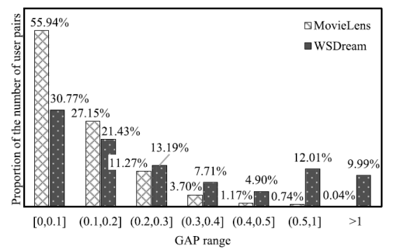
Fig. 1. Distribution proportions of user pairs in different GAPs. If two users of MovieLens have a big similarity, they are more likely to make similar evaluations for the same movies, while two users of WSDream may observe very different QoS values on their commonly invoked web services even they have a high similarity.
图1.不同GAP中用户对的分布比例。 如果MovieLens的两个用户具有很大的相似性,则他们更可能对相同的电影进行类似的评估,而WSDream的两个用户可能在他们通常调用的Web服务上观察到非常不同的QoS值,即使它们具有高相似性。
From Fig. 1 we can see that UPM has many more user pairs than UPW in GAPs of [0, 0.1] and (0.1, 0.2], while UPW has more user pairs than UPM in other GAPs where the two users of one pair may have very different experiences on one item. Also worth attention is there are 9.99 percent user pairs of UPW have GAPs greater than 1, which means that these user pairs may bring errors greater than 100 percent in the predictions of traditional CF. Fig. 1 suggests us that if two users of MovieLens have a big similarity then they are likely to make similar evaluation for their common movies, while two users of WSDream may get very different QoS values on the same web services even they have a big similarity.
We have also observed the item pairs in MovieLens and WSDream by the similar way above, which suggests us that even the high similar web services may give very different QoS values to same users.
Why are MovieLens and WSDream such different as Fig. 1 showed? Our preliminary speculation suggests that, with subjective datasets, such as movie scores, if two audiences have seen many similar movies, then they have similar tastes, and therefore their evaluation of a movie will be similar. But it isn’t true for objective data, which is not created by user. Objective data (e.g., web service QoS values) is created by objective factors beyond user.
从图1可以看出,UPM在[0,0.1]和(0.1,0.2]的GAP中具有比UPW更多的用户对,而UPW在其他GAP中具有比UPM更多的用户对,其中一对中的两个用户可以在一个项目上有非常不同的经验。另外值得注意的是,有9.99%的UPW用户对的GAP大于1,这意味着这些用户对可能会在传统CF的预测中带来大于100%的错误。图1建议我们如果MovieLens的两个用户具有很大的相似性,那么他们很可能对他们的普通电影进行类似的评估,而WSDream的两个用户可能在相同的Web服务上获得非常不同的QoS值,即使它们具有很大的相似性。
我们还通过上述类似的方式观察了MovieLens和WSDream中的项目对,这表明即使是高类似的Web服务也可能为相同的用户提供非常不同的QoS值。
为什么MovieLens和WSDream如图1所示不同?我们的初步推测表明,对于主观数据集,例如电影配乐,如果两个观众看过许多类似的电影,那么他们的口味相似,因此他们对电影的评价将是相似的。但对于不是由用户创建的客观数据而言,情况并非如此。客观数据(例如,Web服务QoS值)由超出用户的客观因素创建。
For unknown web service QoS values prediction, most existing CF methods are based the following two equations:
对于未知的Web服务QoS值预测,大多数现有的CF方法基于以下两个方程:
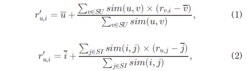
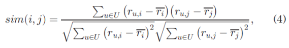
where (1) is user-based CF, (2) is item-based CF, rv;i is the QoS value of service i observed by user v, ru;i’ denotes the prediction of the unknown QoS value ru;i, SU is the set that consists of all users similar to user u, u is the average QoS value of all the services accessed by u, SI is the set of all services similar to service i, i is the average QoS value of i according to all users, sim(u,v) is the similarity between users u and v, and sim(i,j) is the similarity between services i and j. The above two equations (or their improved transformations) play an important role in existing CF-based methods.
其中(1)是基于用户的CF,(2)是基于项目的CF,rv; i是用户v,ru观察到的服务i的QoS值; ru;i’ 表示未知QoS值 ru;i的预测, SU是由与用户u相似的所有用户组成的集合,u是u访问的所有服务的平均QoS值,SI是与服务i类似的所有服务的集合,i是i的平均QoS值。 所有用户,sim(u,v)是用户u和v之间的相似性,而sim(i,j)是服务i和j之间的相似性。 上述两个方程(或其改进的变换)在现有的基于CF的方法中起着重要作用。
However, (1) and (2) work well only if there is no GAP problems. Take (1) for example, if user u and v have a large GAP, then u and v would be very different, and the prediction value r0u;i would be unreasonable. Most existing CF-based methods either just employ this two equations directly [4], [6], [8], [47] or make some reforms but without substantial improvements [3], [5], [7], [9], [45], [46].
但是,只有在没有GAP问题的情况下,(1)和(2)才能正常工作。 以(1)为例,如果用户u和v具有大的GAP,则u和v将是非常不同的,并且预测值r0u; i将是不合理的。 大多数现有的基于CF的方法要么直接使用这两个方程[4],[6],[8],[47],要么进行一些改进但没有实质性的改进[3],[5],[7],[9] ],[45],[46]。
Generally, normalization methods are often used to avoid the GAP problem, but we cannot do this for web service QoS data because another important difference between subjective and objective data. Normalization methods are used mainly if we know the maximum and minimum values of the data. In most subjective datasets, all the values are fixed in a known value scope. For example, all the rating scores of MovieLens are fixed in the scope of [1, 5]. However, it is difficult to determine the QoS values scope of web services since the constantly appearing of new added users and web services, and the scope of QoS value often changes. We have made statistics on the changed QoS value scope for WSDream. There are 1,831,253 and 1,873,838 QoS values (got from 339 users on 5,825 web services, and the missing values are eliminated) in the two of WSDream datasets, i.e., throughput and response time dataset respectively. We surveyed how much the new added QoS values exceed the old QoS value scopes before it added. If a web service give a suddenly changed QoS value for its new added user (from user0 to user338) and the new QoS value exceed its old value scope more than 100 percent then this value is recorded. There are total 12,827 and 12,962 such QoS values for all the web services in throughput and response time datasets, respectively. This means that each user would encounter about 40 web services on average who give them a suddenly changed QoS value. Notice that the original WSDream datasets are very dense which reduces the changes of QoS values scope. In practice, the datasets are often spare and the changes of QoS value scope are more serious with the appearing of new users and web services. Since we cannot known the fixed QoS value scope, the normalization methods are difficult to be employed to avoid the GAP problem.
通常,规范化方法通常用于避免GAP问题,但我们不能对Web服务QoS数据执行此操作,因为主观数据和客观数据之间存在另一个重要差异。如果我们知道数据的最大值和最小值,则主要使用规范化方法。在大多数主观数据集中,所有值都固定在已知值范围内。例如,MovieLens的所有评级分数都固定在[1,5]的范围内。但是,由于新添加的用户和Web服务不断出现,很难确定Web服务的QoS值范围,并且QoS值的范围经常发生变化。我们已经对WSDream的QoS值范围进行了统计。两个WSDream数据集中分别有1,831,253和1,873,838个QoS值(来自5,825个Web服务上的339个用户,并且缺少值被消除),即吞吐量和响应时间数据集。我们调查了新添加的QoS值在添加之前超过旧QoS值范围的程度。如果Web服务为其新添加的用户(从user0到user338)突然更改了QoS值,并且新QoS值超过其旧值范围超过100%,则会记录此值。吞吐量和响应时间数据集中的所有Web服务总共分别有12,827和12,962个这样的QoS值。这意味着每个用户平均会遇到大约40个Web服务,这些服务会给他们一个突然改变的QoS值。请注意,原始WSDream数据集非常密集,这减少了QoS值范围的更改。在实践中,数据集通常是备用的,随着新用户和Web服务的出现,QoS值范围的变化更加严重。由于我们无法知道固定的QoS值范围,因此很难采用规范化方法来避免GAP问题。
From what is mentioned above, traditional CF may not work well for web service QoS prediction, due to the GAP problem which is difficult to avoid by normalization methods. Table 1 illustrates how traditional CF lose efficacy in such case.
Table 1 presents some throughput values in WSDream observed by five users on eight real-world web services from the WSDream dataset. Ui denotes the ith user and WSj denotes the jth web service. If we assume user U242 has never invoked service WS7, then the throughput value is unknown, and it is predicted to be 49.33 by (1) and 49.22 by (2). The prediction errors are caused by the GAPs between U242 and other users, also the GAPs between WS7 and other web services. However, it is difficult to avoid the GAP problem by normalizing the QoS values since the U242-WS7 invocation will give a throughput value exceedingly beyond the old QoS value scopes of U242 ([0.965, 19.672]) and WS7 ([43.337, 112.277]).
从上面提到的,由于归一化方法难以避免的GAP问题,传统CF可能不适用于Web服务QoS预测。 表1说明了传统CF在这种情况下如何丧失功效。
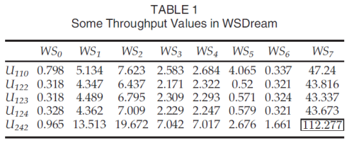
表1显示了五个用户在WSDream数据集中对八个真实Web服务观察到的WSDream中的一些吞吐量值。 Ui表示第i个用户,WSj表示第j个Web服务。 如果我们假设用户U242从未调用过服务WS7,则吞吐量值是未知的,并且通过公式(1)预测为49.33和通过公式(2)为49.22。 预测错误是由U242与其他用户之间的GAP以及WS7与其他Web服务之间的GAP引起的。 但是,通过规范化QoS值很难避免GAP问题,因为U242-WS7调用将使吞吐量值超出U242([0.965,19.672])和WS7([43.337,112.277]的旧QoS值范围。)。
Web service QoS values are objective and have no subjective features, therefore we cannot predict the unknown objective QoS values as for movie scores.
The existing CF based prediction methods for unknown QoS values have not realized the above differences between subjective and objective data and therefore cannot predict objective QoS values accurately. In allusion to this problem this paper presents a highly accurate prediction algorithm (HAPA) for unknown web service QoS values. HAPA is also CF-based, i.e. also use similar users and similar items to make prediction, but with fundamental changes from traditional CF approaches to adapt to the characteristics of objective QoS data. Fig. 1 points out one of the characteristics of objective QoS data, i.e. a high similarity does not means that two users or items present similar QoS values, but this characteristic doesn’t tell us how predict unknown QoS values. Therefore we have to explore other characteristics of objective QoS data which are the theoretical basis of HAPA. These characteristics will tell us what the similarity means to objective QoS data, which can be summarized as: 1) if two users share a high similarity, then their similarity will hardly fluctuate with their future invocations of more numbers of web services, and 2) in the same way, if two items share a high similarity, then their similarity will hardly fluctuate with their future invocations by more numbers of users. We built our HAPA for the prediction of the unknown web service QoS values based on these characteristics which were found by many experiments.
Web服务QoS值是客观的,没有主观特征,因此我们无法像预测电影分数一样预测未知的客观QoS值。
现有的基于CF的未知QoS值预测方法尚未实现主观和客观数据之间的上述差异,因此无法准确预测客观QoS值。针对这个问题,本文提出了一种针对未知Web服务QoS值的高度准确的预测算法(HAPA)。 HAPA也是基于CF的,即也使用类似的用户和类似项目进行预测,但是从传统CF方法的基本变化来适应客观QoS数据的特征。图1指出了客观QoS数据的一个特征,即高相似性并不意味着两个用户或项目呈现相似的QoS值,但是这个特征并没有告诉我们如何预测未知的QoS值。因此,我们必须探索客观QoS数据的其他特征,这些是HAPA的理论基础。这些特征将告诉我们相似性对客观QoS数据意味着什么,可以概括为:1)如果两个用户共享高相似性,那么它们的相似性几乎不会随着他们将来调用更多数量的Web服务而波动,并且2)同样,如果两个项目具有很高的相似性,那么它们的相似性几乎不会随着更多用户的未来调用而波动。我们构建了HAPA,用于根据许多实验发现的这些特征预测未知Web服务QoS值。
The main contributions of this paper are threefold. First, based on real web service QoS data and a number of experiments, we find some important characteristics of objective QoS datasets that have never been found before. Second, we propose a web service QoS value prediction algorithm HAPA to realize these characteristics, allowing the unknown QoS values to be predicted accurately. Finally, we conduct several real world experiments to verify our prediction accuracy.
The rest of this paper is organized as follows. Section 2 presents our highly accurate prediction algorithm for unknown web service QoS values and also analyze its computational complexity. Section 3 describes our experiments. Section 4 shows related work, and Section 5 concludes the paper.
本文的主要贡献有三个方面。 首先,基于真实的Web服务QoS数据和大量实验,我们发现了以前从未发现的客观QoS数据集的一些重要特征。 其次,我们提出了一种Web服务QoS值预测算法HAPA来实现这些特性,允许准确地预测未知的QoS值。 最后,我们进行了几次真实的实验,以验证我们的预测准确性。
本文的其余部分安排如下。 第2节介绍了我们针对未知Web服务QoS值的高度准确的预测算法,并分析了其计算复杂性。 第3节描述了我们的实验。 第4节显示相关工作,第5节结束本文。
2 PROPOSED HAPA
HAPA is a CF-based algorithm, i.e., it concretely consists of user-based and item-based HAPAs. Each type of HAPA can make predictions, however we always use the combination of the two HAPAs to make predictions more accurate.
This section first presents the theoretical foundation of HAPA, then introduce the mechanisms of user-based and item-based HAPAs, and finally describe how make predictions employing the combination of the two HAPAs.
2提出HAPA
HAPA是基于CF的算法,即,它具体地包括基于用户和基于项目的HAPA。 每种类型的HAPA都可以进行预测,但是我们总是使用两种HAPA的组合来使预测更准确。
本节首先介绍了HAPA的理论基础,然后介绍了基于用户和基于项目的HAPA的机制,最后描述了如何使用两个HAPA的组合进行预测。
2.1 Theoretical Foundation of HAPA
In this section we carry out some analysis of the characteristics of QoS data based on which we propose our HAPA.
We use PCC to measure the similarity between users or items. For user-based CF methods, PCC uses the following equation to calculate the similarity between two users u and v based on the web services they commonly invoke:
在本节中,我们基于我们提出的HAPA对QoS数据的特征进行了一些分析。
我们使用PCC来衡量用户或项目之间的相似性。 对于基于用户的CF方法,PCC使用以下等式根据他们通常调用的Web服务计算两个用户u和v之间的相似性:
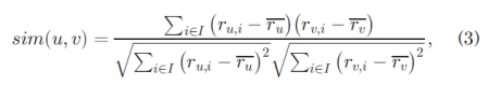
where is the subset of web service previously invoked by both user u and v. ru;i is the QoS value of web service i observed by user u, and ru represents the average QoS value of different web services observed by user u. Similarly, for item-based CF, the PCC between two service items is calculated as:
其中是用户u和v先前调用的Web服务的子集; ru;i 是用户u观察到的Web服务的QoS值,ru表示用户u观察到的不同Web服务的平均QoS值。
同样,对于基于项目的CF,两个服务项之间的PCC计算如下:
where U =Ui ∩Uj is the subset of users who have previously invoked both web services i and j, and ri represents the average QoS value of web service i observed by different users.
We adopt WSDream datasets to carry out analysis. WSDream contains two 339*5825 user-item matrixes. Each value is the response time for a user invoking a web service in a matrix, and the throughput for a user invoking a web service in another matrix.
其中U =Ui∩Uj是先前已调用Web服务i和j的用户的子集,ri表示不同用户观察到的Web服务的平均QoS值。
我们采用WSDream数据集进行分析。 WSDream包含两个339 * 5825用户项矩阵。 每个值是用户在矩阵中调用Web服务的响应时间,以及用户在另一个矩阵中调用Web服务的吞吐量。
We want to study how the similarity between two users or web services changes with the growing user-service invocations. In this study, we found that if two users have a high similarity, then their similarity will hardly fluctuate with their growing invocations of web services. On the contrary, if two users have only a low similarity, then their similarity would fluctuate notably with their growing invocations of web services. The same phenomenon can be found for the similarity between web services. If two web services have a high similarity, then their similarity will hardly fluctuate with their growing invocations by users. Conversely, if two web services have only a low similarity, then their similarity would fluctuate notably with their growing invocations by users. We have made statistics of all user and web service pairs on the entire WSDream datasets to verify these phenomenon, which is shown as Fig. 2. We got Fig. 2 as the following five steps:
我们想研究两个用户或Web服务之间的相似性如何随着不断增长的用户服务调用而变化。 在这项研究中,我们发现,如果两个用户具有很高的相似性,那么他们的相似性几乎不会随着他们对Web服务的不断增长的调用而波动。 相反,如果两个用户的相似度很低,那么他们的相似性会随着他们对Web服务的不断增长的调用而显着波动。 对于Web服务之间的相似性,可以发现相同的现象。 如果两个Web服务具有高度相似性,那么它们的相似性几乎不会随着用户的不断增长的调用而波动。 相反,如果两个Web服务只具有较低的相似性,那么它们的相似性会随着用户的不断增长的调用而显着波动。 我们在整个WSDream数据集上对所有用户和Web服务对进行了统计,以验证这些现象,如图2所示。我们将图2作为以下五个步骤:

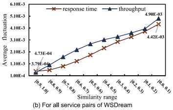
Fig. 2. Average fluctuation in each similarity range, which suggests us a characteristic of PCC similarity: the higher the similarity the steadier the similarity and vice versa.
图2.每个相似性范围的平均波动,这表明我们具有PCC相似性的特征:相似性越高,相似性越稳定,反之亦然。
- Randomly remove some invocation values from the two datasets of WSDream until only 5 percent invocation entries left. (As we can’t know the actual situations of the future user-service invocations, we deleted some invocations from the dataset. Then the dataset with more deletions denotes “the past”, and the dataset with less or no deletions denotes “the future”.)
- We divide the two datasets of WSDream (it is very sparse now) on the similarity basis, i.e., [0, 0.1), . . ., [0.9, 1]. For each similarity range, we find out all the user pairs whose similarity belong to this range.
- For each user pair (u, v), we randomly add a web service to Iu ∩Iv. We can know this service’s QoS values (for user u and v) from the original dataset, and then the change of similarity simeu; vT is calculated out. The absolute value of the difference in similarity is used to denote the fluctuation. This step is repeated until all web services are added to Iu ∩ Iv.
4) We calculated the average fluctuation of similarity of all user pair for each similarity range.
5) We treat all the service pairs of each similarity range in the similar way above.
1)从WSDream的两个数据集中随机删除一些调用值,直到只剩下5%的调用项。 (由于我们无法知道未来用户服务调用的实际情况,我们从数据集中删除了一些调用。然后具有更多删除的数据集表示“过去”,而删除较少或没有删除的数据集表示“未来”。)
2)我们在相似性基础上划分WSDream的两个数据集(现在它非常稀疏),即[0,0.1),. 。 。,[0.9,1]。对于每个相似性范围,我们找出其相似性属于该范围的所有用户对。
3)对于每个用户对(u,v),我们随机向Iu ∩Iv添加Web服务。我们可以从原始数据集中了解该服务的QoS值(对于用户u和v),然后计算出是相似性sim(u,v)的变化。相似度差的绝对值用于表示波动。重复此步骤,直到将所有Web服务添加到Iu∩ Iv。
4)我们计算了每个相似范围的所有用户对的相似度的平均波动。
5)我们以类似的方式处理每个相似范围的所有服务对。
Since Step 1 make the datasets sparse of 5 percent density, Fig. 2 can represents the feature of WSDream in different matrix density from 5 percent to about 90 percent (The density of original response time and throughput datasets are 94.9 and 92.7 percent respectively), because the density increases with the adding process.
From Fig. 2 we can see that if user u and v have a high similarity, then this similarity will hardly change with their future invocations of more web services, and in the same way, the higher the similarity two services have, the steadier the similarity with their future invocations by more numbers of users. Then we propose the following two characteristics of QoS data:
由于步骤1使数据集稀疏度为5%,图2可以表示WSDream在不同矩阵密度下的特征,从5%到约90%(原始响应时间和吞吐量数据集的密度分别为94.9和92.7%), 因为密度随着添加过程而增加。
从图2中我们可以看到,如果用户u和v具有高度的相似性,那么这种相似性将随着他们将来调用更多Web服务而变化,并且以相同的方式,两个服务具有的相似性越高,越稳定,与更多用户的未来调用相似。 然后我们提出了QoS数据的以下两个特征:
Characteristic 1. For two pairs of service users (u; v) and(u0; v0), if sim(u; v) is considerably greater than sim(u0; v0), then sim(u; v) will fluctuate less than sim(u0; v0) when they invocate more web services.
Characteristic 2. For two pairs of services (i; j) and (i0; j0), if sim(i; j) is considerably greater than sim(i0; j0), then sim(i; j) would fluctuate less than sim(i0; j0) when they are invocated by more users.
We can use Characteristics 1 and 2 to derive Corollaries 1 and 2, respectively:
Corollary 1. If we use a high similar user v to predict the unknown QoS value ru;i, then sim(u; v) should hardly change after the prediction of ru;i. This can be explained by Characteristic 1, i.e., predicting ru;i is equivalent to adding a service to Iu ∩ Iv.
Corollary 2. If we use a high similar service j to predict the unknown value ru;i, then sim(i; j) should hardly change after the prediction of ru;i. This can be explained by Characteristic 2, i.e., predicting ru;i is equivalent to adding a user to Ui ∩Uj.
特征1.对于两对服务用户(u; v)和(u0; v0),如果sim(u; v)远大于sim(u0; v0),则sim(u; v)将波动小于sim(u0; v0),当他们调用更多的Web服务时。
特征2.对于两对服务(i; j)和(i0; j0),如果sim(i; j)远大于sim(i0; j0),那么sim(i; j)将比sim小波动(i0; j0)当更多用户调用它们时。
我们可以使用特征1和2分别得出推论1和2:
推论1.如果我们使用高度相似的用户v来预测未知的QoS值ru; i,那么sim(u; v)在预测ru; i之后几乎不会改变。这可以通过特征1来解释,即预测ru; i相当于向Iu∩Iv添加服务。
推论2.如果我们使用高相似服务j来预测未知值ru; i,那么sim(i; j)在预测ru之后几乎不会改变; i。这可以通过特征2来解释,即预测ru; i相当于将用户添加到Ui∩Uj。
These corollaries are the theoretical foundation of our proposed algorithm HAPA. HAPA includes user-based and item-based prediction according to Corollaries 1 and 2, respectively. A detailed explanation of the prediction mechanism is given in Sections 2.2 and 2.3, respectively. To aid the following descriptions, we first give some definitions.
Definition 3 (Active user). The active user is one who requires a prediction for an unknown QoS value.
Definition 4 (Similar user). If an active user u requires the unknown QoS value ru;i and rv;i is already known, then service user v is a similar user to service user u.
Definition 5 (Similar service). If an active user u requires the unknown QoS value ru;i and ru;j is already known, then service j is a similar service to service i.
这些推论是我们提出的算法HAPA的理论基础。 HAPA分别根据推论1和2包括基于用户和基于项目的预测。 预测机制的详细说明分别在2.2节和2.3节中给出。 为了帮助以下描述,我们首先给出一些定义。
定义3(活动用户)。 活动用户是需要预测未知QoS值的用户。
定义4(类似用户)。 如果活动用户u需要未知QoS值ru; i和rv; i已知,则服务用户v是服务用户u的类似用户。
定义5(类似服务)。 如果活动用户u需要未知QoS值ru; i和ru; j已知,则服务j是与服务i类似的服务。
2.2 User-Based HAPA
User-based HAPA consists of three steps: 1) a user-based prediction equation is constructed based on each similar user to mathematically implement Corollary 1; 2) these prediction equations are proved to be quadratic, that produce two prediction values, in which only one value is appropriate, and therefore linear regression is used to select the appropriate prediction value for each prediction equation; 3) the unknown QoS value is calculated from all the prediction values made by every similar user.
2.2基于用户的HAPA
基于用户的HAPA包括三个步骤:1)基于每个相似用户构建基于用户的预测方程,以数学方式实现推论1; 2)这些预测方程被证明是二次的,产生两个预测值,其中只有一个值是合适的,因此线性回归用于为每个预测方程选择合适的预测值; 3)根据每个类似用户做出的所有预测值计算未知QoS值。
2.2.1 User-Based Prediction Equation
The user-based prediction equation is a mathematical formulation of Corollary 1. Before constructing these equations, we first find the top similar users with big similarities. Let user_topK denote the number of these top similar users, and let KU represent the set of these top similar users. In Section 3.4 we study how big the similarity is appropriate by experiments and it determines user_topK.
2.2.1基于用户的预测方程
基于用户的预测方程是推论1的数学公式。在构造这些方程之前,我们首先找到具有大相似性的顶级类似用户。 让user_topK表示这些顶级类似用户的数量,让KU代表这些顶级类似用户的集合。 在3.4节中,我们通过实验研究相似性有多大,并确定user_topK。
Suppose ru;i is the unknown QoS value, and let x represent the predicted value of ru;i. User su is a similar user to u. To establish the prediction equation based on user su, we assume that user u has invoked service i, and let x be the QoS value for this invocation. When the invocation has finished, we recalculate the similarity between user u and su. Let the new similarity be sim0eu; suT. Inspired by Corollary 1, we know that the new similarity sim0eu; suT should be approximately the same as the old similarity simeu; suT. Thus, we have:
假设ru; i是未知的QoS值,并且x表示预测值ru;i。 用户su是与u类似的用户。 为了建立基于用户su的预测方程,我们假设用户u已经调用了服务i,并且x是该调用的QoS值。 调用完成后,我们重新计算用户u和su之间的相似性。 让新的相似度为sim0(u;su)。 在推论1的启发下,我们知道新的相似性sim0(u; su)应与旧的相似性sim(u;su)大致相同。 因此,我们有:

where
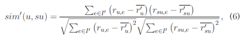
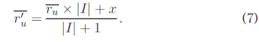
where I0 =I ∪{service i}, because we have assumed that user u has invoked service i. Let x be the QoS value of service i for this invocation by user u. r0u and r0su are the average QoS values of different services observed by users u and su, respectively. Obviously, r0u is a function of x, written as:
其中I' = I∪{service i},因为我们假设用户你已经调用了服务i。令x为用户u对此调用的服务i的QoS值。 r'u和r'su分别是用户u和su观察到的不同服务的平均QoS值。显然,r'u是x的函数,写为:
Therefore, (5) is a function of x, and x is the only variable in (5). Hence, to predict ru;i, we solve for x to satisfy (5).
因此,(5)是x的函数,x是(5)中的唯一变量。因此,为了预测ru; i,我们求x满足(5)。
Substituting the data of users u and su into (6) and substituting (6) into (5) give:
将用户u和su的数据代入(6)而代入(6)代入(5)给出:
where the constant coefficients a, b and c are determined by user u, the constant coefficient d is determined by the similar user su, constant coefficients e and f are commonly determined by user u and the similar user su, and the original similarity simeu; suT is already known. Chen et al. (8) is a user-based prediction equation.
We can easily transform (8) to a quadratic equation. The predicted value of ru;i must be one of the two roots of (8), and we use linear regression to select the appropriate root.
其中常数系数a,b和c由用户u确定,常数系数d由类似用户su确定,常数系数e和f通常由用户u和类似用户su和原始相似度sim(u; su)确定已经知道了。陈等人。 (8)是基于用户的预测方程。
我们可以很容易地将(8)变换为二次方程。 ru的预测值; i必须是(8)的两个根之一,我们使用线性回归来选择适当的根。
2.2.2 Linear Regression for User-Based Prediction Equation
Linear regression can be used to predict a vector based on another linearly related vector. As we are using PCC to measure the similarity and choosing highly similar users to make predictions, user u and the similar user su should have a strong linear relationship. Therefore, we can use linear regression to make a rough prediction, and then use the rough prediction to select the appropriate root.
We establish the linear regression model as:
2.2.2基于用户的预测方程的线性回归
线性回归可用于基于另一线性相关矢量来预测矢量。 由于我们使用PCC来测量相似性并选择高度相似的用户来进行预测,因此用户u和类似用户su应该具有强烈的线性关系。 因此,我们可以使用线性回归进行粗略预测,然后使用粗略预测来选择合适的根。
我们建立线性回归模型:

where b0 and b1 represent coefficients of the linear relationship between user u and similar user su. Using the two coefficients, we obtain a rough prediction of ru;i as:
其中b0和b1表示用户u和类似用户su之间的线性关系的系数。 使用这两个系数,我们得到ru的粗略预测; i为:

where rpsu( ru;i) is the rough prediction of ru;i made by similar user su. Let x1 and x2 denote the two roots of the user-based prediction equation (8). We select the appropriate root as follows:
中rpsu(ru; i)是ru的粗略预测是由类似的用户su制作的。 令x1和x2表示基于用户的预测方程(8)的两个根。 我们选择适当的根如下:
where presu(ru;i) is the predicted value of ru;i made by the the similar user su.
其中presu(ru;i)是由类似的用户su得到的ru的预测值。
2.2.3 Final Prediction for User-Based HAPA
After each similar user in KU calculating out a prediction value using its prediction equation and linear regression, we would have user_topK prediction values. Now we should determine the final accurate prediction by comprehensively considering all the similar users of KU as follow:
在KU中的每个类似用户使用其预测方程和线性回归计算出预测值之后,我们将具有user_topK预测值。 现在我们应该通过综合考虑KU的所有类似用户来确定最终的准确预测如下:
where r^u;i is the final prediction of ru;i, and con(su) denotes the confidence in the prediction given by su. Because a higher similarity generally gives greater stability, we will obtain a more accurate prediction from users with a higher similarity. Therefore, we have more confidence in users who have a higher similarity to user u. This can be written as:
其中r ^ u; i是ru的最终预测; i,con(su)表示su给出的预测的置信度。 因为较高的相似性通常会提供更高的稳定性,我们将从具有更高相似性的用户获得更准确的预测。 因此,我们对与用户u具有更高相似性的用户更有信心。 这可以写成:

2.3 Item-Based HAPA
(略)
2.4 Make Prediction via HAPA
Though each of user-based and item-based HAPAs can make prediction, HAPA combines this two kinds of HAPAs to further improve the prediction accuracy.
2.4通过HAPA进行预测
虽然每个基于用户和基于项目的HAPA都可以进行预测,但是HAPA结合了这两种HAPA来进一步提高预测精度。
Let ru,i be the unknown QoS value, pvuser and pvitem denote the predicted values given by user-based and item-based HAPA respectively. We use the following three indexes to evaluate the quality of these predicted values:
设ru,i是未知的QoS值,pvuser和pvitem分别表示基于用户和基于项目的HAPA给出的预测值。
我们使用以下三个索引来评估这些预测值的质量:
- Max similarity (MS). For pvuser and pvitem, MS represents the maximum similarity between users in KU and services in KI, denoted by ms(pvuser) and ms(pvitem), respectively.
2)Average similarity (AS). For pvuser and pvitem, AS represents the average similarity between users in KU and services in KI, denoted by asepvuserT and asepvitemT, respectively.
3) Reciprocal of standard deviation (RSD). For pvuser and pvitem, RSD represents the reciprocal of the standard deviation of the similarities between users in KU and services in KI, denoted by rsd(pvuser) and rsd(pvitem), respectively.
These indexes can be written as:
1)最大相似度(MS)。 对于pvuser和pvitem,MS表示KU中的用户与KI中的服务之间的最大相似度,分别由ms(pvuser)和ms(pvitem)表示。
2)平均相似度(AS)。 对于pvuser和pvitem,AS表示KU中的用户与KI中的服务之间的平均相似度,分别由asepvuserT和asepvitemT表示。
3)标准偏差(RSD)的倒数。 对于pvuser和pvitem,RSD表示KU中的用户与KI中的服务之间的相似性的标准偏差的倒数,分别由rsd(pvuser) 和rsd(pvitem)表示。
这些索引可以写成:

If we decompose the prediction quality into each index, then we have:
如果我们将预测质量分解为每个索引,那么我们有:

The prediction quality of pvuser and pvitem can then be obtained as:
然后可以获得pvuser和pvitem的预测质量:
Hence, the final predicted value of ru;i is:
3 EXPERIMENTS
In this section, we perform experiments to validate our HAPA, and compare the results with those from other CF methods. Our experiments are intended to: 1) verify the rationality of our proposed characteristics and corollaries; 2) compare HAPA with other CF methods; and 3) parameterize HAPA to achieve optimum performance.
3、实验
在本节中,我们将进行实验以验证我们的HAPA,并将结果与其他CF方法的结果进行比较。 我们的实验旨在:1)验证我们提出的特征和推论的合理性; 2)将HAPA与其他CF方法进行比较; 3)参数化HAPA以达到最佳性能。
3.1 Experiments Setup
We adopted WSDream to validate our prediction algorithm. We implemented the experiments employing JDK 7.0 and eclipse 4.3 on Windows Server 2008 R2 Enterprises with Inter Xeon E5-2670 eight-core 2.60 GHz CPU and 32 G RAM. Our experiments mainly consists of two parts: 1) Section 3.3 compares our algorithm with other seven well known prediction methods based on the throughput as well as response time dataset; 2) Sections 3.4 and 3.5 study the optimal parameters user_topK and item_topK of our algorithm.
To validate the accuracy of our algorithm, we predict only the known values, so that we can evaluate the error between the predicted values and real values.
3.1实验设置
我们采用WSDream来验证我们的预测算法。 我们使用InterXeon E5-2670八核2.60 GHz CPU和32 G RAM在Windows Server 2008 R2企业上实施了采用JDK 7.0和eclipse 4.3的实验。 我们的实验主要由两部分组成:1)3.3节将我们的算法与其他七种众所周知的预测方法进行比较,这些预测方法基于吞吐量和响应时间数据集; 2)第3.4和3.5节研究了算法的最佳参数user_topK和item_topK。
为了验证算法的准确性,我们只预测已知值,以便我们可以评估预测值和实际值之间的误差。
3.2 Accuracy Metrics
The mean absolute error (MAE) and root mean squared error (RMSE) are frequently used to measure the difference between values predicted by a model or estimator and observed values. We adopted MAE and RMSE to measure the prediction accuracy of our algorithm through comparisons with other methods. MAE is defined as: 3.2准确度指标
平均绝对误差(MAE)和均方根误差(RMSE)经常用于测量由模型或估计器预测的值与观测值之间的差异。 我们采用MAE和RMSE通过与其他方法的比较来测量算法的预测精度。 MAE定义为:

where Rij denotes the QoS value of service j observed by user i, b Rij is the predicted QoS value, and N is the number of predicted values.
RMSE is defined as:
其中Rij表示用户i观测到的服务j的QoS值,b Rij是预测的QoS值,N是预测值的数量。
RMSE定义为:
This is a good measure of accuracy when comparing prediction errors from different models for a particular variable [16].
当比较特定变量的不同模型的预测误差时,这是一种很好的准确度[16]。
3.3 Comparisons
We compare the predictive performance of our HAPA with other seven well known prediction methods. The seven compared methods are follows:
1) UMEAN (user mean). UMEAN employs the average QoS value of a user to predict the unknown QoS values.
2) IMEAN (item mean). IMEAN uses the average QoS value of the web service from other users to predict the unknown QoS values.
3) UPCC (user-based collaborative filtering method using PCC). UPCC employs similar users for the QoS value prediction [9], [17].
4) IPCC (item-based collaborative filtering method using PCC). IPCC employs similar web services (items) for the QoS value prediction [18].
5) UIPCC. This method combines UPCC and IPCC for the QoS value prediction [4].
6) Nonnegative matrix factorization (NMF). NMF was proposed by Lee and Seung [19], [20]. It is different from other matrix factorization methods, as it enforces the factorized matrices to be nonnegative.
7) Probabilistic matrix factorization (PMF). PMF was proposed by Salakhutdinov and Minh [21], and employs a user-item matrix for recommendations. PMF is based on probabilistic matrix factorization.
3.3比较
我们将HAPA的预测性能与其他七种众所周知的预测方法进行了比较。七种比较方法如下:
1)UMEAN(用户意思)。 UMEAN使用用户的平均QoS值来预测未知的QoS值。
2)IMEAN(项目均值)。 IMEAN使用来自其他用户的Web服务的平均QoS值来预测未知的QoS值。
3)UPCC(使用PCC的基于用户的协同过滤方法)。 UPCC使用类似的用户进行QoS值预测[9],[17]。
4)IPCC(使用PCC的基于项目的协同过滤方法)。 IPCC采用类似的Web服务(项目)进行QoS值预测[18]。
5)UIPCC。该方法将UPCC和IPCC结合起来用于QoS值预测[4]。
6)非负矩阵分解(NMF)。 NMF由Lee和Seung提出[19],[20]。它与其他矩阵分解方法不同,因为它强制分解矩阵是非负的。
7)概率矩阵分解(PMF)。 PMF由Salakhutdinov和Minh [21]提出,并使用用户项矩阵作为推荐。 PMF基于概率矩阵分解。
Sparse matrixes are common in the real word, and accurate predictions for sparse matrixes are very important in many practical applications, such as recommender systems, social networking, and so on. In this experiment, we made the datasets sparser by removing entries, enabling us to compare HAPA with the other methods using various dataset densities. The experimental results are shown in Table 2.
稀疏矩阵在真实世界中是常见的,并且稀疏矩阵的准确预测在许多实际应用中非常重要,例如推荐系统,社交网络等。 在这个实验中,我们通过删除条目使数据集更稀疏,使我们能够使用各种数据集密度将HAPA与其他方法进行比较。 实验结果如表2所示。
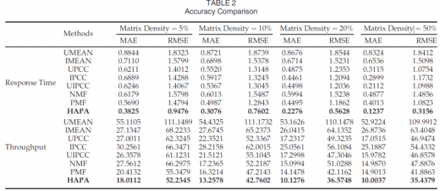
From Table 2, we can see that HAPA is more accurate than all of the other methods for all the two datasets. As the matrix density increases from 5 to 50 percent, the MAE and RMSE values become smaller, because the similarities between different users or different services become steadier as the amount of data increases.
从表2中,我们可以看到HAPA比所有这两个数据集的所有其他方法更准确。 随着矩阵密度从5%增加到50%,MAE和RMSE值变小,因为随着数据量的增加,不同用户或不同服务之间的相似性变得更稳定。
3.4 Impact of User_topK
3.4.1 Is the Bigger User_topK the Better?
We employed user-based HAPA, i.e., only similar users, to predict 1,000 known values of the dataset with different values of user_topK. Fig. 3 shows the resulting prediction accuracies. Note that smaller values of MAE and RMSE are better. Fig. 3 indicates that user_topK ?10, 50, 100, 150, 200, 250, 300, 330 gives relatively accurate predictions. However, when user_topK exceeds 150, the prediction accuracy declines quickly. We believe that this is because, when user_topK becomes too large, users with very low similarity are employed to make predictions. To avoid this problem, a good user_topK should exclude small similarities. As stated in Characteristic 2, if active user u and the similar user v are not very similar, then their similarity may fluctuate noticeably when they invoke more services, and the prediction equation no longer be valid. Hence, when user_topK ?330 (in a dataset containing 339 users), the high number of low similarity between users causes large prediction errors (see Fig. 3).
This experiment suggests us that user_TopK is not the bigger the better. To find the optimum user_topK, we designed the following experiment.
3.4 User_topK的影响
3.4.1 Bigger User_topK更好吗?
我们使用基于用户的HAPA,即仅使用类似用户来预测具有不同user_topK值的数据集的1,000个已知值。图3显示了最终的预测精度。请注意,较小的MAE和RMSE值更好。图3表示user_topK?10,50,100,150,200,250,300,330给出相对准确的预测。但是,当user_topK超过150时,预测精度会迅速下降。我们认为这是因为,当user_topK变得太大时,使用具有非常低相似性的用户进行预测。为了避免这个问题,一个好的user_topK应该排除很小的相似之处。如特征2中所述,如果活动用户u和类似用户v不是非常相似,则当它们调用更多服务时它们的相似性可能明显波动,并且预测方程不再有效。因此,当user_topK≥330(在包含339个用户的数据集中)时,用户之间的高数量的低相似性导致大的预测误差(参见图3)。

这个实验告诉我们user_TopK不是越大越好。为了找到最佳的user_topK,我们设计了以下实验。
3.4.2 The Optimum Setting of User_topK
To study the optimum value of user_topK, i.e., the number of similar users needed to give a relatively accurate prediction, we studied one active user at a time.
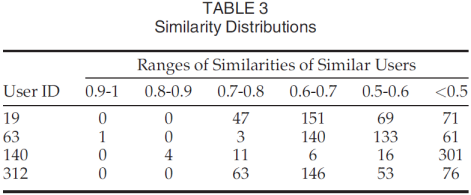
We have speculated that the optimum user_topK is related to the similarity distribution. Therefore, we first studied the distribution of similarities for active users before making predictions, and observed the similarity ranges of the user_topK most similar users. Table 3 shows the results for four users selected from the dataset. User ID in Table 3 denotes the row number of the dataset, i.e., a user can be recognized as a row of the matrix. For each of the four users, we calculated how many similar users exist in different similarity ranges.
Based on these similarity distributions, we examined which similarity ranges provided the most accurate predictions.
3.4.2 User_topK的最佳设置
为了研究user_topK的最佳值,即,给出相对准确的预测所需的类似用户的数量,我们一次研究了一个活动用户。
我们推测最佳user_topK与相似度分布有关。 因此,我们首先在进行预测之前研究了活跃用户的相似性分布,并观察了user_topK最相似用户的相似性范围。表3显示了从数据集中选择的四个用户的结果。 表3中的用户ID表示数据集的行号,即,用户可以被识别为矩阵的行。 对于四个用户中的每一个,我们计算了在不同相似性范围中存在多少相似用户。
基于这些相似性分布,我们检查了哪些相似性范围提供了最准确的预测。
For each user of Table 3, we predicted 500 values shown as Fig. 4. Combining Table 3 and Fig. 4, we obtain a clear picture of the similarity ranges that contribute to accurate predictions.
From Fig. 4a, the most accurate prediction for user 19 comes from user_topK ?200. User 19 has 198 similar users whose similarity is greater than 0.6. Therefore, it is these users who contribute to the prediction accuracy.
Fig. 4b shows that very few, highly similar users can give a relatively accurate prediction. When user_topK ?4, we obtained a prediction accuracy for user 63 with MAE ?0.6 and RMSE ?1.5. As user_topK increased from 4 to 150, most similar users appear in the similarity range [0.6, 0.7], and these give the best prediction accuracy. Increasing user_topK to 200 introduced similar users in the similarity range [0.5, 0.6], and these harmed the prediction accuracy.
User 140 has only 21 similar users whose similarity is greater than 0.6. The additional 16 users in the similarity range [0.5, 0.6] improved the prediction accuracy slightly (see Fig. 4c), suggesting that users with a similarity value above 0.5 have an uncertain effect on prediction accuracy, as they caused the prediction accuracy of users 4 and 63 to deteriorate.
Similarly, user 312 obtained good prediction accuracy from user_topK ?200 with almost all the similar users whose similarity is greater than 0.6 (see Fig. 4d).
Fig. 4 tells us that a similarity greater than 0.6 contributes to accurate prediction, and that similarities around 0.5 are unreliable.
Thus, this experiment suggests that the optimum value of user_topK is determined by the similarity distribution of similar users. For different active users, the best user_topKs are different. High performance can be achieved by setting user_topK to introduce all similar users whose similarity value is above 0.6.
对于表3的每个用户,我们预测500个值如图4所示。结合表3和图4,我们获得了有助于准确预测的相似性范围的清晰图像。
从图4a中,对用户19的最准确预测来自user_topK?200。用户19具有198个相似用户,其相似度大于0.6。因此,正是这些用户对预测准确性做出了贡献。
图4b显示极少数,高度相似的用户可以给出相对准确的预测。当user_topK≥4时,我们用MAE≤0.6和RMSE≤1.5获得用户63的预测精度。随着user_topK从4增加到150,大多数类似用户出现在相似性范围[0.6,0.7]中,并且这些用户提供了最佳的预测准确性。将user_topK增加到200引入了相似范围[0.5,0.6]中的类似用户,并且这些损害了预测准确性。
用户140只有21个相似用户,其相似度大于0.6。相似范围[0.5,0.6]中的另外16个用户略微提高了预测精度(参见图4c),表明相似值大于0.5的用户对预测准确性具有不确定的影响,因为它们导致用户的预测准确性4和63恶化。
类似地,用户312从user_topK?200获得了良好的预测精度,其中几乎所有类似用户的相似度都大于0.6(参见图4d)。
图4告诉我们,大于0.6的相似性有助于准确预测,并且0.5左右的相似性是不可靠的。
因此,该实验表明user_topK的最佳值由类似用户的相似性分布确定。对于不同的活动用户,最佳user_topKs是不同的。通过设置user_topK以引入相似值大于0.6的所有类似用户,可以实现高性能。
3.5 Impact of Item_topK
The mathematical principle of user-based HAPA is identical to that of item-based HAPA, as both users and services are processed as arrays of the two-dimensional QoS dataset. However, most services in the dataset have many very similar services (similarity greater than 0.9), unlike users, for whom similarity greater than 0.8 are rare. Hence, we studied how high similarity scores affect the item_topK setting. When using item-based HAPA to make predictions, we find it interesting that relatively few (about 10) highly similar services (similarity greater than 0.9) can give an accurate prediction.
As shown in Table 4, we selected four services that have a number of highly similar services. Service ID denotes the column occupied by that service in the dataset. We predicted 100 known QoS values for each of the four services under different item_topK values. The prediction accuracies are shown in Table 5. From Table 5, we can see that the prediction accuracy barely changed as item_topK increased. These results conform to Characteristic 2, as two very similar services have a steady similarity, and therefore, after predicting a QoS value for a service, the predicted value should not affect this similarity. Thus, we do not need many highly similar services to make accurate predictions.
This is in contrast to user-based HAPA, where we generally required a large value of user_topK. To illustrate this, if we let ANU [a, b) denote the average number of similar users whose similarity is in the interval [a, b) for each user, and let ANS [a, b) denote the average number of similar services whose similarity is in the interval [a, b) for each service, then ANU [0.9, 1) ?0.41, ANS [0.9, 1) ?41.35, and ANU [0.8, 0.9) ?4.07, ANS [0.8, 0.9) ?104.89.
3.5 Item_topK的影响
基于用户的HAPA的数学原理与基于项目的HAPA的数学原理相同,因为用户和服务都被处理为二维QoS数据集的数组。但是,数据集中的大多数服务都有许多非常相似的服务(相似度大于0.9),与用户不同,相似度大于0.8的情况很少见。因此,我们研究了高相似度得分对item_topK设置的影响程度。当使用基于项目的HAPA进行预测时,我们发现有趣的是相对较少(约10个)高度相似的服务(相似度大于0.9)可以给出准确的预测。
如表4所示,我们选择了四种具有大量高度相似服务的服务。服务ID表示该服务在数据集中占用的列。我们在不同的item_topK值下预测了四种服务中的每一种的100个已知QoS值。预测精度如表5所示。从表5中可以看出,随着item_topK的增加,预测精度几乎没有变化。这些结果符合特征2,因为两个非常相似的服务具有稳定的相似性,因此,在预测服务的QoS值之后,预测值不应影响该相似性。因此,我们不需要许多高度相似的服务来进行准确的预测。
这与基于用户的HAPA形成对比,我们通常需要较大的user_topK值。为了说明这一点,如果我们让ANU [a,b)表示每个用户的相似度在区间[a,b)中的相似用户的平均数量,并且让ANS [a,b]表示类似服务的平均数量其相似性在每个服务的区间[a,b),然后ANU [0.9,1]?0.41,ANS [0.9,1]?41.35和ANU [0.8,0.9]?4.07,ANS [0.8,0.9) ?104.89。
3.6 Combining User-Based and Item-Based HAPAs Can Make Prediction More Accurate
HAPA use the combination of user-based and item-based HAPAs to make prediction more accurate. Based on the experiments of Sections 3.4 and 3.5, we have determined good values for user_topK and item_topK. These parameters values are dynamic with the number of the similarities greater than 0.6. For example, if we need to predict ru;i, user_topK should be set as follows:
- For user u, if there exist more than 10 users with similarities greater than 0.9, then we can directly set user_topK =10. Of course, we can set a larger value, but this will have a small effect on the prediction accuracy.
- If there are not enough similar users with similarities greater than 0.9, we set the value of user_topK to the number of users whose similarity is at least 0.6.
3.6结合基于用户和基于项目的HAPA可以使预测更准确
HAPA使用基于用户和基于项目的HAPA的组合来使预测更准确。 根据第3.4节和第3.5节的实验,我们确定了user_topK和item_topK的良好值。 这些参数值是动态的,相似数大于0.6。 例如,如果我们需要预测ru; i,user_topK应该设置如下:
1)对于用户u,如果有超过10个相似度大于0.9的用户,那么我们可以直接设置user_topK = 10。 当然,我们可以设置更大的值,但这对预测精度影响很小。
2)如果没有足够相似的用户,其相似度大于0.9,我们将user_topK的值设置为相似度至少为0.6的用户数。
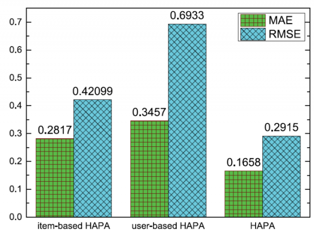
The setting of item_topK is similar. Using the user-based HAPA, item-based HAPA and their combination, we predicted 10,000 QoS values. A comparison of the prediction accuracy is shown in Fig. 5.
From Fig. 5, the HAPA clearly gives the most accurate predictions. HAPA employed user-based and item-based HAPAs to obtain two prediction values, and then, using the three indexes MS, AS, and RSD proposed in Section 2.4, evaluated the quality of these predicted values to form the final prediction. Therefore, HAPA gives more accurate predictions than either user-based or item-based HAPA.
item_topK的设置类似。 使用基于用户的HAPA,基于项目的HAPA及其组合,我们预测了10,000个QoS值。 预测精度的比较如图5所示。
从图5中,HAPA清楚地给出了最准确的预测。 HAPA采用基于用户和基于项目的HAPA来获得两个预测值,然后,使用2.4节中提出的MS,AS和RSD三个指标,评估这些预测值的质量以形成最终预测。 因此,HAPA比基于用户的或基于项目的HAPA提供更准确的预测。
5 CONCLUSION AND FUTURE WORK
We have utilized CF to predict unknown QoS values. Strictly speaking, our approach is essentially different from traditional CF which is not applicable to objective data prediction.
Traditional CF is based on the premise that similar users have similar subjective experience on the same items, but this premise no longer applies for the objective data. By the way of experiments, we determined some important characteristics of PCC similarity first. These characteristics show that the magnitude of PCC similarity determines its stability. Based on these characteristics, we proposed our HAPA. The prediction accuracy of HAPA was shown to outperform that of many of existing QoS prediction methods.
As the definition of Objective Data, web service QoS is determined as a result of some objective factors, such as network traffic, bandwidth, when and where a user accessed a web service. Our proposed HAPA does not predict unknown QoS values by these objective factors, but directly by the known QoS values. We can make predictions even more accurately if we know the relationship between these objective factors and the final QoS. To work out this relationship, we still have some important problems to solve, such as finding the core objective factors, how observe these objective factors, how probe user context and how learn this relationship. We are trying to solve these problems and will propose our approaches in the future work.
5结论和未来的工作
我们利用CF来预测未知的QoS值。严格地说,我们的方法与传统的CF本质上不同,后者不适用于客观数据预测。
传统CF基于类似用户对相同项目具有相似主观体验的前提,但此前提不再适用于客观数据。通过实验,我们首先确定了PCC相似性的一些重要特征。这些特征表明PCC相似性的大小决定了它的稳定性。基于这些特点,我们提出了HAPA。 HAPA的预测精度显示出优于许多现有QoS预测方法的预测精度。
作为目标数据的定义,Web服务QoS是由一些客观因素决定的,例如网络流量,带宽,用户访问Web服务的时间和地点。我们提出的HAPA不会通过这些客观因素预测未知的QoS值,而是直接通过已知的QoS值来预测。如果我们知道这些客观因素与最终QoS之间的关系,我们就能更准确地做出预测。为了解决这种关系,我们仍然需要解决一些重要问题,例如找到核心客观因素,如何观察这些客观因素,如何探索用户背景以及如何学习这种关系。我们正在努力解决这些问题,并将在未来的工作中提出我们的方法。
本文链接:https://my.lmcjl.com/post/19297.html
4 评论